
,
,
, , , , 06, 05, 04, 03, 02, 01,
0000000000000
Formatting Fonts: Formatting Toolbar
Formatting Fonts: Formatting Palette
Formatting Numbers: Toolbar Option
Formatting Numbers: Menu Option
Merging and Centering Text: Toolbar Option
Merging and Centering Text: Menu Option
Unmerging Text: Toolbar Option
Wrapping Text: Keyboard Option
Begin a new folder – 12 – 12 in your Excel Folder
Word > Two > Excel > 12 - 12
You will end up with six saved Worksheets by the time you have completed Exercise One.
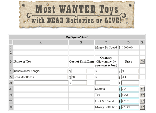
Fill out at least ten items in the online ‘Toy Spreadsheet’ and save it to your folder for today.
In Excel > Open File > Templates (in the rightside panel) > On My Computer > Spreadsheet Solutions
Open each template and fill data (for example some description - date - figures) do at least three lines for each one then save it in Word > Two > Excel > 12 - 12 as the name of the template. For example, BalanceSheet-1
Exercise One B
Start a new 'Worksheet' and save it in your Word > Two > Excel > 12 - 12 folder as 'color'. Change the color coding in the cells, the text (you will need to write text such as the months across the top), the tabs, the background, and the grids. If you can not find how to do it in Format > Cells then go to the Help menu and look it up. For example, 'color code' > view 'Add color to sheet tabs'.
Exercise One C
Fill in the online form below with enough toys to equal $1000 and save it in your Word > Two > Excel > 12 - 12 folder as 'toys'.
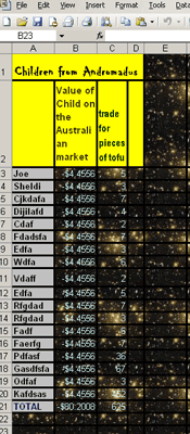
Spreadsheets come in all types and things. For example, look at this easy to use online type of spreadsheet:
Using your own original data - This will be an added to follow the dots type of thingy with an end result that will appear something like:
Working with large amounts of data can make one go around the bend and come back with brain damage if it is not done properly. One of the ways to make data management easier is to organize your workbook into different worksheets. Planning the design of your workbook from the start can make it easier to work with, especially when the workbook gets larger or contains several sections and gets into the thousands as we will. For example, worksheets within your current collection of dolls can be color coded (text, cells, or background) to differentiate among class sections; even the worksheet tabs can be color coded. Other things we will merrily learn to do to make organizing our data more efficient will (but will not be limited to) include the following:
To make formatting worksheets a little tinny bit easier, Excel has bequest us with several "preset" formats available. If you recall we went through this with Word and Publisher and of course we will discover that there are formats (templates) for many other products – sometimes it seems as the whole day is just one large template (which of course it is) – chosen by your teacher, parents, the government... With these preset formats, you can select all of the characteristics or only some (e.g., just the borders). Once you apply the formatting with AutoFormat, you can still make adjustments to the cells.
1. Select the cell(s) to be formatted
2.
From the Format menu, select AutoFormat...
The AutoFormat dialog box appears.
3. Select the desired AutoFormatting option
b. Under Formats to apply, select/deselect the desired options
5. Click OK
Two options for formatting fonts in Excel are the Formatting toolbar option and the Format menu option. The Format Cells dialog box contains many other style choices not available on the Formatting toolbar.
Windows:
![]()
1. Select the cell(s) to be formatted
2.
On the Formatting toolbar, click the desired formatting option
NOTES:
Holding the pointer over a toolbar button for a short period displays a
description of that option.
If the desired option is not available on the Formatting toolbar, refer
to Formatting Font:
Menu Option - below.
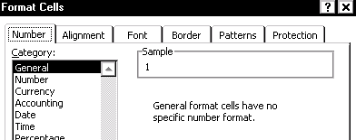
In addition to font choices, the Format Cells dialog box contains many other style choices that are not available on the Formatting toolbar.
1. Select the cell(s) to be formatted
2.
From the Format menu, select Cells…
The Format Cells dialog box appears.
3. Select the Font tab
4. Make the desired changes
5. Click OK Formatting Numbers
Formatting cells for numbers can be very helpful and time-saving. You can format cells to display time, currency, numbers, etc. in the desired style.
![]()
1. Select the cell(s) to be formatted
2.
On the Formatting toolbar, click the desired formatting option
NOTES:
Holding the pointer over a toolbar button for a short period displays a
description of that option.
1. Select the cell(s) to be formatted
2.
From the Format menu, select Cells…
The Format Cells dialog box appears.
3.
Select the Number tab
NOTE: Under Category, you will see some
common choices for formatting numbers.
4.
From the Category scroll box, select the appropriate number
category
Based on your selection, additional options appear.
5. Make the appropriate choices
6. Click OK
1. Select the cell(s) to be formatted
2.
From the Format menu, select Cells...
The Format Cells dialog box appears.
3. Select the Number tab
4. From the Category scroll box, select Date
5.
From the Type scroll box, select the desired four-digit year
option
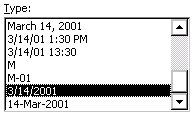
6. Click OK
Merging and centering text in your Excel document can add a professional appearance. Merging and centering is useful for titles and headings so they are not broken up into different cells or displayed with inappropriate alignment.
1. Type the desired text in the first cell of the group to be merged
2.
Select the text and a cell from each column you want merged
EXAMPLE: To center across columns A through
D in row 2 of the worksheet, select cells A2, B2, C2, and D2
3.
On the Formatting toolbar, click MERGE AND CENTER![]()
1. Type the desired text in the first cell of the group to be merged
2.
Select the text and a cell from each column you want merged
EXAMPLE: To center across columns A through
D in row 2 of the worksheet, select cells A2, B2, C2, and D2
3.
From the Format menu, select Cells…
The Format Cells dialog box appears.
4. Select the Alignment tab
5.
From the Horizontal pull-down list, select Center Across
Selection
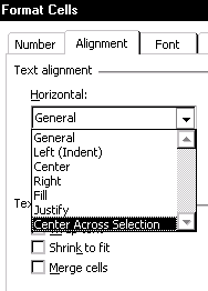
6. Under Text control, select Merge cells
7. Click OK
1. Select the merged cell
2.
On the Formatting toolbar, click MERGE AND CENTER![]()
1. Select the merged cell
2.
From the Format menu, select Cells...
The Format Cells dialog box appears.
3. Select the Alignment tab
4. From the Horizontal pull-down list, select General
5. Under Text control, deselect Merge cells
6. Click OK
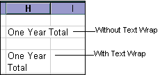
We did this yesterday but do it again today so you have it perfect. If you
have text that appears in a single cell and you want to increase the height of
that cell to accommodate all of the words, you can use the Wrap text
option.
1. Select the cells to which Wrap text will be applied
2.
From the Format menu, select Cells…
The Format Cells dialog box appears.
3. Select the Alignment tab
4. Under Text control, select Wrap text
5.
Click OK
The text is wrapped.
NOTE: To display all of the text, it may be
necessary to adjust row height.
1. Select the cells
2. In the Formula Bar text box, place the insertion point where Wrap text will be applied
3.
Windows: Press [Alt] +
[Enter]
Macintosh: Press [control] +
[option] + [return]
The text is wrapped.
1. Select the cell containing wrapped text
2.
From the Format menu, select Cells...
The Format Cells dialog box appears.
3. Under Text control, deselect Wrap text
4.
Click OK
The text is unwrapped.
The typical Copy and Paste function will copy the information (e.g., text, formula) and the formatting of the cell(s). If you want to copy only the formatting, you can use the Painter option. This will format the destination cell the same as the source cell without changing the content.
If you want to remove all formatting from a cell but leave the contents (e.g., text, value, formulas), use the following command.
1. Select the cell(s) containing the formatting to be cleared
2. From the Edit menu, select Clear » Formats