JUMP TO Today
computer classes homepage 8b Moodle / Wiki / My Dwight /Trimester Two youtube project
Trimester Three
When your poem is finished (including music background) it will be here > http://www.youtube.com/poem4photo
May 16th Day 5 Friday Period 1
TASK - Five lines five images or more. Firstly, do each of your lines as text in Photoshop with a background then we will animate them. Examples saved as .gif (reason.gif; tango.gif and tango-tween.gif) then save your finished work as a movie (.avi format).
When you have all your layers done deselect all your layers (click the eye)
Go to Window > Animation > 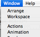 Click in the corner of the frame panel
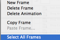
 ![]() and select all frames
and select all frames
 >
>
Export your final product (file > Export > movie) 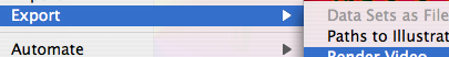
ASSESSMENT - Create a movie of your poem and put it in the grade eight folder (click anywhere on your desktop > Click GO at the top menu [![]() ] and group 2012 [
] and group 2012 [ ] and drag your NAME-poem-1.mov into the poetry folder.
So at the end of your project you will see it on youtube like this at our page with the user name "poem4photo" our group is called 'Picture Poems'
May 12 Monday Day 1
The day you have been waiting for, Poetry days. Here are some ideas. Start today with putting some words (perhaps the first dozen) onto a path. We will be adding several techniques then be creating an animated poem. Some examples are in the Here are some ideas. section
May 2 Friday Day 1 Go to the website http://www.xist.org/earth/pop_region.aspx and
1. Create a chart similar to the one below
2. Take the continents out of the stats and what is the largest country - the smallest?
3.
Choose the data from the same site on male-female differences (Male/female distribution) by country. Using sort which country has the largest gender ratio? Which country has the most female to male ratio? What is it? What country has the highest and which the lowest children born?
April 30th Wednesday Day 5
ASSESSMENT - (read below) For your grade today
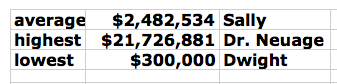
1. See below (http://roadsidephotos.sabr.org/baseball/data.htm) then Print ONLY the sheet with the following data on it: average salary, highest salary and lowest salary with the players name next to it. Be sure your name is on the paper.
2. From the URL http://en.wikipedia.org/wiki/List_of_highest_paid_baseball_players go to "2007 Annual Salaries" make a chart (HINT put the data in three columns first) and print the page with your chart on it including a heading on the chart.
Functions are done in the order that they are written:
=(B11+B20)/6 For example, in this order the cells are added then divided by six
=(B11*B20)^2
=10*((B11+B20) -- (B30+B40))
So far we have written =sum for our formula then divided by the number of cells to get our average. We can also write =average to get our result. For example, instead of =SUM(B45:B72)/26 key in =AVERAGE(B45:B72) to get our average of $77.79.
The parameters of a function are called arguments. Each function name is followed by parentheses, which contain its arguments. Even functions that require no arguments must still have the parentheses after the name, as in =TODAY().
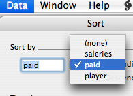
Calculating Min > You can use the MIN function to find the lowest number in a series of numbers. In our data it is between =MAX(B45:N74)
DAY 3 -April 28th Monday - Day 3 From the website Business of Baseball Downloadable Data and Documents I have placed ticket price spreadsheets in your gmail accounts. Find the average prices of tickets over the years included and then select four teams and create a chart. 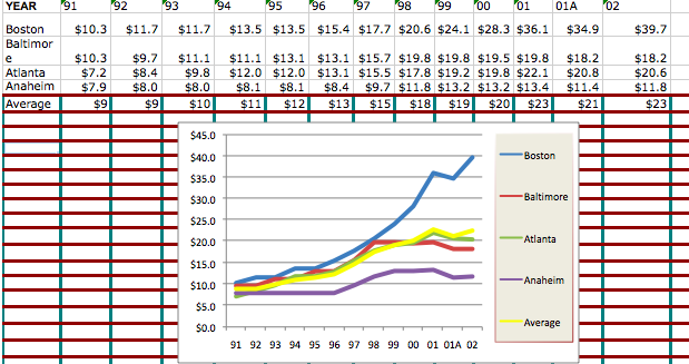
Be sure you have printed in handed in your two charts for genre and years for the music that this class listens to. Save your work as we will be coming back to this.
TASK - Learning functions. The parameters of a function are called arguments.
Formulas begin with an equal sign. Following the = sign is (sum). Your formula can include cell references, fixed numbers, and math operators for addition (+), subtraction ( - ), multiplication (*), division (/), and exponentiation (^). For example, =(B1+B97)/14
=(B1*B97)^2
=10*((B1+B5)- -- (B3+B7))
ASSESSMENT -


April 11 Day 5 As I am at a workshop today please follow these instructions. If you have questions use the help file.
Continue with putting your data in for your songs in the year's sheet and the genre sheet. Be sure you have your standard and formatting tools visible > 
1. Taking your "years" sheet copy (highlight and copy) the rows with years and numbers which you may have taken from your song's sheet or if you wrote them onto a paper then put in the numbers. ![]()
2. In a column following your years write "total songs" ![]() and wrap the text -
and wrap the text - 
3.
Highlight the row of numbers of songs (not the years) and using the autosum add them (click autosum whilst having the cell you are putting the data in selected)  so you have the total number of songs in the correct cell >
 ![]()
4. Do the same for genres and put your totals on your genre page. You may wish to do as you did with the years and put several types of music in your top row and put in a number following each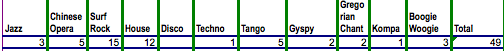
5. Next we will make charts. In Excel 2008 for Mac that we are using you may have noticed that there is a new icon menu (called The Ribbon) across the top.![]() Click each and have a bit of a play with them to see what they do - or better yet - what you do with them. Be sure to explore the sub-menus also. We are using Blank Sheets, the first one for this assignment.
Click each and have a bit of a play with them to see what they do - or better yet - what you do with them. Be sure to explore the sub-menus also. We are using Blank Sheets, the first one for this assignment. ![]()
If you have created lots of additional sheets whilst looking at the various menus please delete all but your three sheets: songs, years, genres - thanks mate. ![]() =
= ![]()
6. Charts. Charts show our data. We need to be sure our year's labels have words as well as the year. If we just have the decades then Excel will interpret this as numbers =  and this tells us nothing. Therefore, put songs after the year =
 ![]() .
.
A. Highlight your two rows and try out different charts, for example (as it is close to lunch I chose "pie" charts)  To get the percent double click on the chart you chose which will open the "Format Data Point" and click "labels" > and "show percent" as well as ticking the "Show legend key next to label" box.
Be sure that your name is on the sheet then print (being careful to only print the one sheet and not all the others) your page with at least two different charts showing your data. If you finish doing the years then do the same with genres. When you have completed these two sheets you may have free time. Cheers Dr. Neuage
ASSESSMENT -
April 3 Thursday Day 5 printed notes
Follow these steps:
1.
Open your Gmail spreadsheet for the music sheet
2. Export the music spreadsheet as .xls 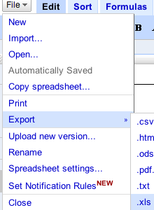
3. Open the sheet in Excel
4. If you have already started a spreadsheet for your music project open that and copy your Gmail sheet into it. If you have not started your project then add two more sheets 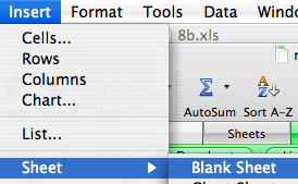 and label your sheet tabs
 ![]() the listSONGS is your sheet from Gmail:
the listSONGS is your sheet from Gmail:
5. Add these columns to your spreadsheet (years page) ![]()
6. Go through the songs and create column labels of the different genres (types) of music in the list - there may be four or five more types. For example: 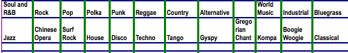
7. How many songs are in each category?
8. As there are 49 song selections (some are duplicates) you need to have them equal your total (49) in the last column - you will need to write "total" in the last column. For example, 
9. Highlight the two rows (do this in for each sheet; the one for genres and the one for years) and experiment with the different tapes of charts available at the top of the Excel page: 
select ONE chart that best demonstrates your data - use a different chart on each page. 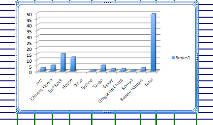
DAY 3 - Tuesday April 1st To create a spreadsheet of favorite songs ---
1. grades from last projects
2. Today TASK - Firstly using Google Docs - spreadsheets list - write in column one five songs you know are popular as well as their singer. 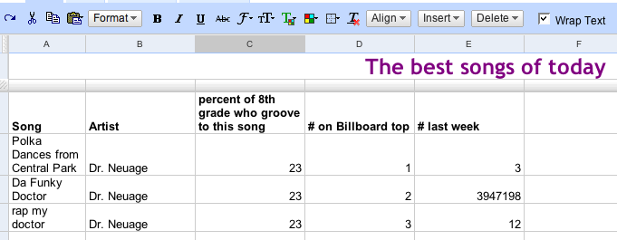 After doing that open Excel in Office 2008 and set up a worksheet saved as "Music-List" - include an image as a background and the following headings:
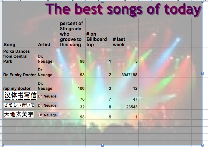
Next class, you will gather the data from the Google Spreadsheet and put into your individual Excel sheet and follow the next steps then.
You will need to move the transparency slider to make the background lighter... (under format picture or double click on the image = ![]()
A.
songs
B.
artist
C.
current #/last week#/how many weeks on charts/
3. ASSESSMENT -
THURSDAY 12h DAY 5
1. TASK - Complete exercise of four slides - an extra slide receives extra credit. Anyone touching someone else's slides loses points.
2. ASSESSMENT - Four slides on your Social Studies work. Mr. Theisen will grade the content I will grade the technology sections. To get credit you must share it with others - or at least me. DrNeuage@gmail.com.
When you are finished do the exercise in Moodle.
MONDAY 10th - DAY 3
1. TASK - Go to your gmail account and if you did not get your invite for this lesson from me speak up (not too loudly).
2. ASSESSMENT - Four slides on your Social Studies work. Mr. Theisen will grade the content I will grade the technology sections. This will be a two lesson exercise.
TUESDAY 4TH DAY 5
1. TASK To collaborate on a presentation
2. ASSESSMENT Check your gmail. You need to create two related to the topic slides for five points. Include text as well as an image. 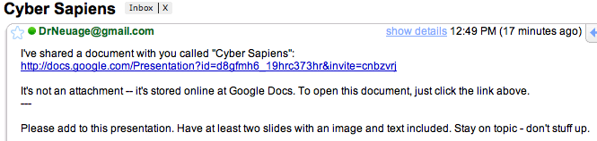
THURSDAY 28th - DAY 3
1. TASK Watch this video clip then (putting your first name before what you write) write in Google Documents (check your gmail) "Episode 9 Manipulating Society through Technology" of your thoughts on the level society is being manipulated with technology. Ten points. Go to http://www.devsource.com/c/s/Videos/
Scroll down to 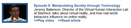
2. ASSESSMENT To have written something about this clip in your google documents. Five points.
FRIDAY 22ND DAY 5
1. TASK To share a document with all those in our class. Continuing with Google applications - Open Documents
A. We will collect everyone's email address so that we can work on a document together - See Moodle
B. Open
2. ASSESSMENT
A. Answer the Google questions - six points
B. Have written something in our Google Document and "shared it with those in our class - including me (DrNeuage@gmail.com) - four points. 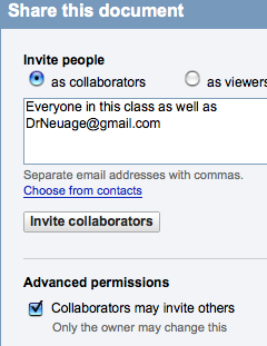
WEDNESDAY 20th - DAY 3
1. TASKs - Details how to do this are below
a.
To create a Google Notebook with a folder for each class
b. To add this site to your technology folder as well as your notes for trimester three
2. ASSESSMENT - This assignment is worth ten points toward your final grade
a. Five points for your folders which should look something like this - of course you will list all your classes 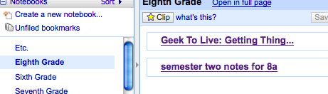
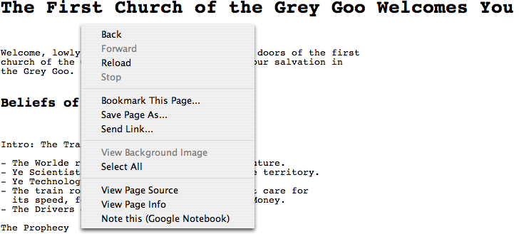
ABOUT Google Notebook http://www.google.com/notebook - a good way to save what you find on the Internet into folders accessible anywhere (on earth). Sign onto Google and click notebook or go to notebook in a Google search = http://www.google.com/notebook
1. Set up a google notebook and for assessment set up a folder for each of your classes. Find something on the Internet that you will add to your folder. For example, if I had a class in Nanotechnology I would make a folder "Nanotechnology" and if I wanted to add something I found on nanotechnology Gray Goo right click or on a mac book ctrl click and if you have downloaded notebooks you will see "Note this (Google Notebook)" as shown below then put it in the correct folder;